Nanite All The Things

A whole lot has changed in Unreal in the last few years, I’ve found it interesting to look back over all the things I wanted in the software, and how rapidly it has been advancing.

My obsession with wanting real time edge weighted subdivision surfaces in the engine, for example, has backed off substancially thanks to Nanite!

Nanite does an incredible job of compressing assets, especially if you use Trim Relative Error even a little.
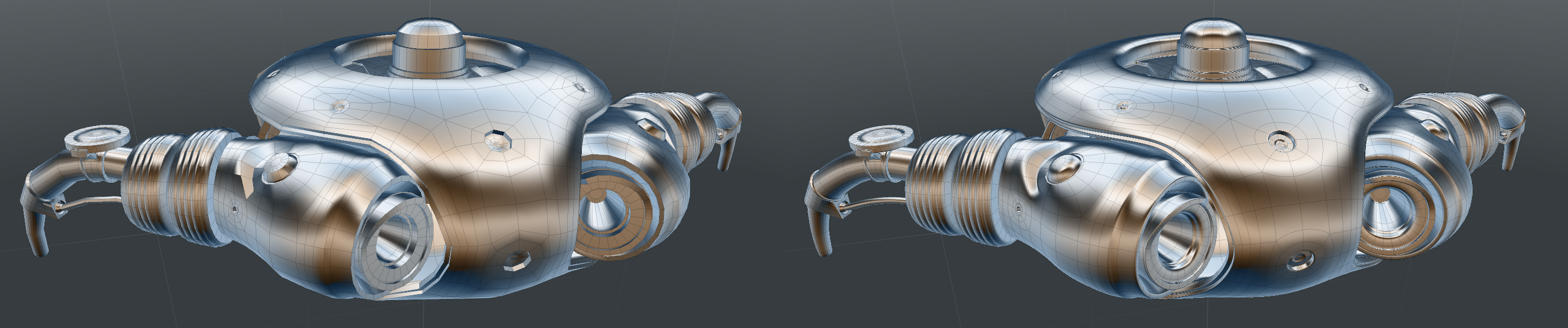
For example, this little robot doodad thingo is about 560 Kb in edge weighted sub-d in Modo:

Subdivide that and import it into Unreal as Nanite, and it is about 90 Mb, but trim relative error takes it down to 5mb, with minimal visual difference:

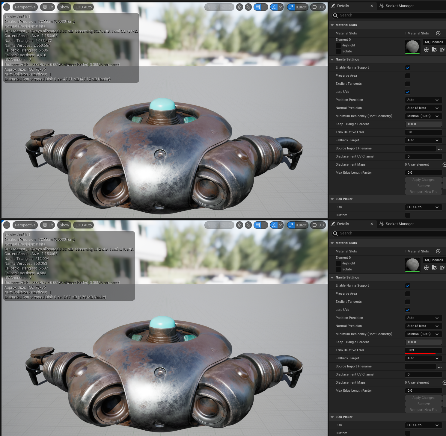
That mesh is still 10x as big as the sub-d Modo source file.

But whatever you ended up doing to get sub-d working in realtime, you’d be paying some non-zero memory cost for that subdivided asset, unless you are straight up raytracing the limit surface and not generating the triangles at all. And even *if* that is a feasible thing, I have no idea what other costs you’d have…

So yes fine, Nanite has incredible compression, and might get me over my realtime sub-d hangups 😛

Nanite Tessellation rocks!

In 5.4 we get Nanite Tessellation!

It has been demo’d very well in the GDC State of Unreal in the new Marvel Rise of Hydra game, the Preview is out, so I’ve had a few days playing 🙂

It has also been discussed in a bunch of recent videos from Epic that I still need to get around to finding and watching, and will post in the comments at some point…

Why Tessellation? Lots of reasons, but I’ll start with one I really wanted to try out!

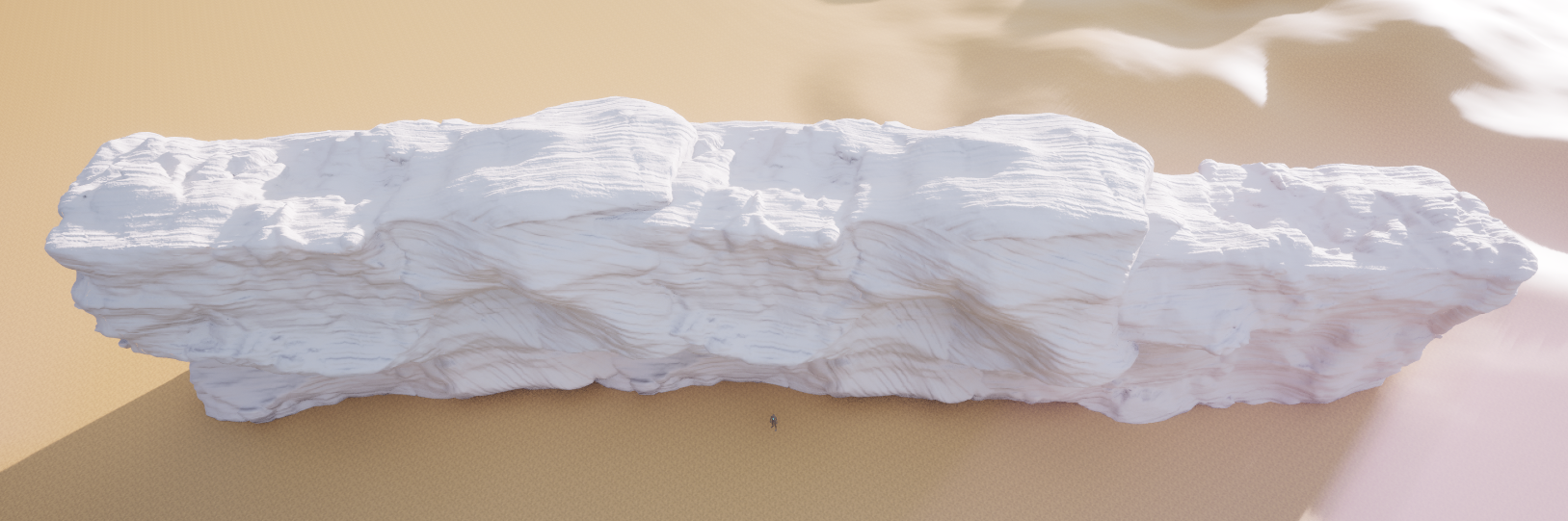
So imagine you want to make a 20m high rock cliff in one piece, and have enough ground level vertices for 1st person camera detail, with a vertex every 5 to 10 centimetres. Not really as sensible as building something out of smaller pieces, but not out of the realms of something I’d like to do.

What that looks like in Houdini for my big rock (box for rough human scale):

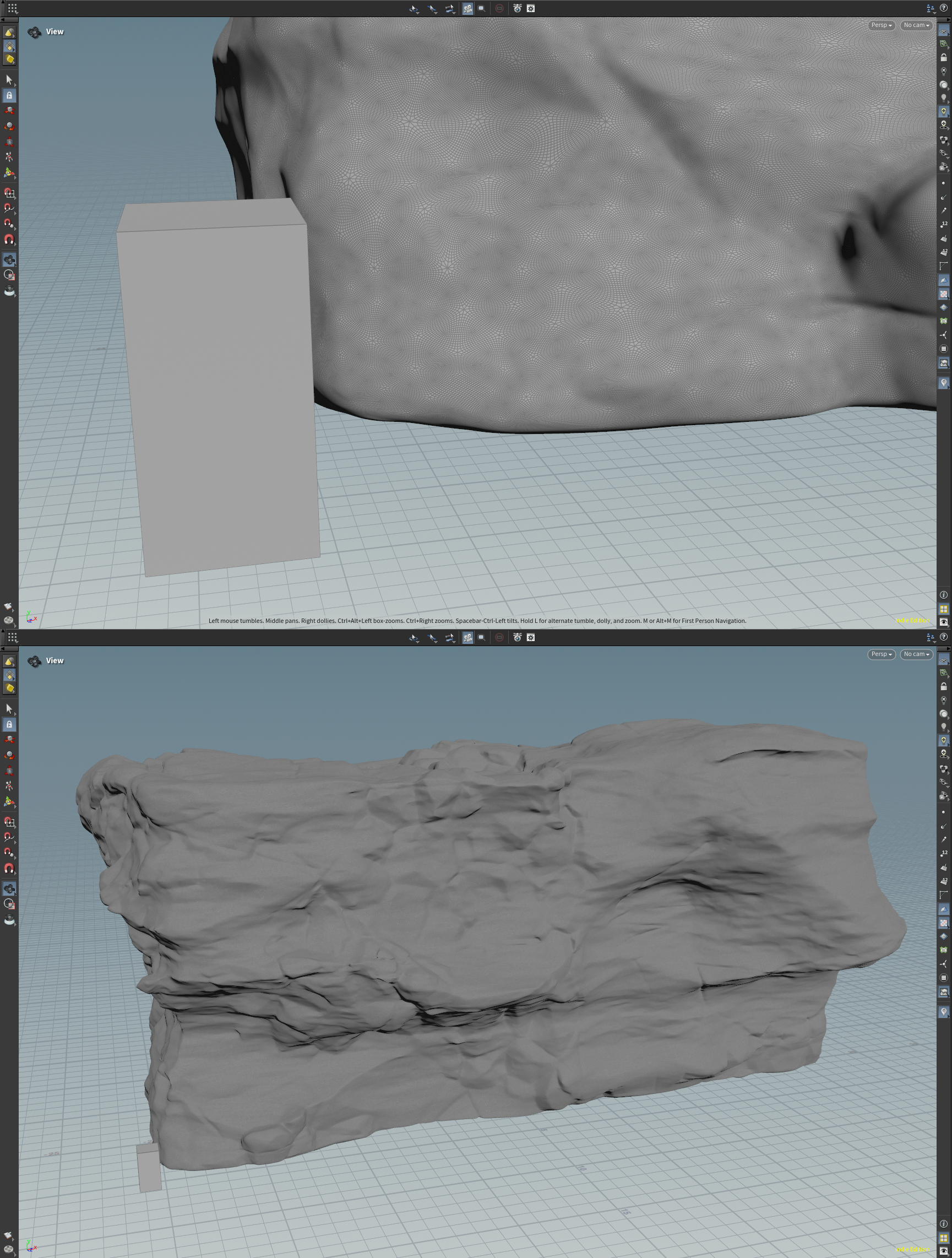
That is a 70 million vertex mesh, and maybe on the light side of things for close up details tbh…

Can you import that as Nanite? Sure, it will take a few minutes just to save the fbx file for it, it will be 4gb, and good luck if you want to UV / texture it…

Artists find sensible ways around this sort of thing: unwrap a lower poly mesh and project the high poly back onto it, use software like Rizom that handles high vertex counts, if you happen to know you will always be ground level, concentrate the vertex data there and have less up top, etc, etc.

Using the Displacement on import options on Static Meshes (that I believe Epic built out for upgrading Fortnite assets to Nanite) is also an option here.

Ignoring that though, importing a mesh this size into Unreal might take 30+ minutes, and you end up with something like this:

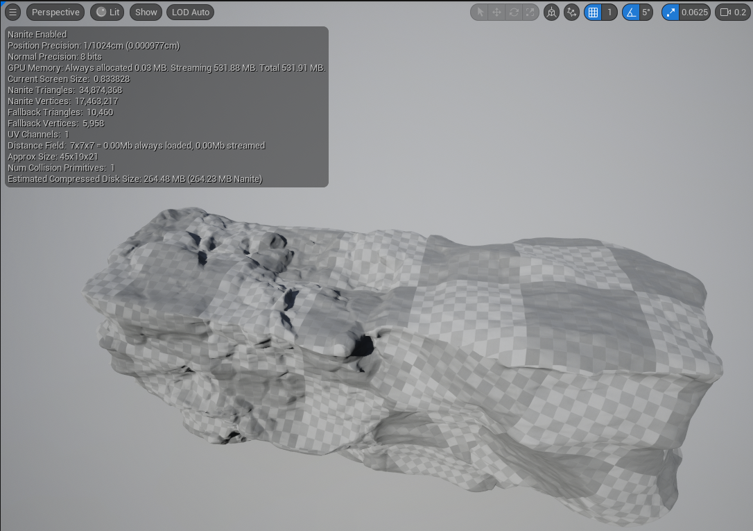
531 Mb is still very impressive for that amount of data!

And entirely reducable using Trim Relative Error, but given it takes a long time to regenerate the mesh you might find yourself spending hours tweaking Trim Relative Error to find the right balance, and you will still be sacrificing detail.

Lower base mesh detail with tiling displacement

Nanite Tessellation gives us another approach that gives us lower resolution assets to work with in DCC tools like Houdini and Modo, but also the opportunity to create more generic tilable displacement that can be used across multiple assets.

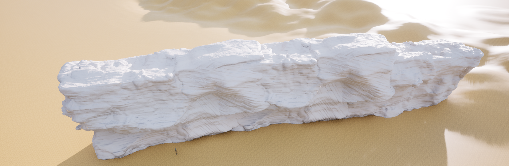
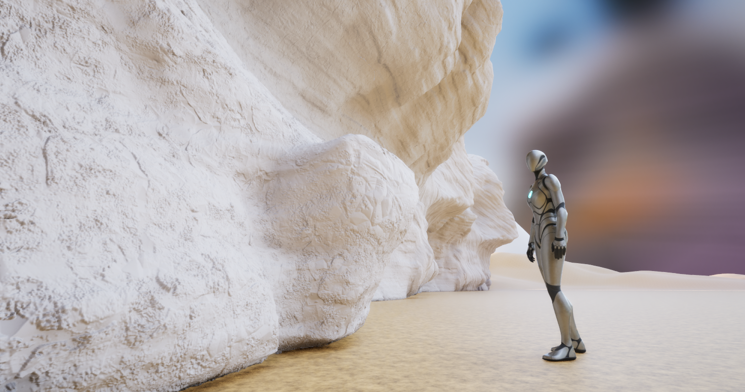
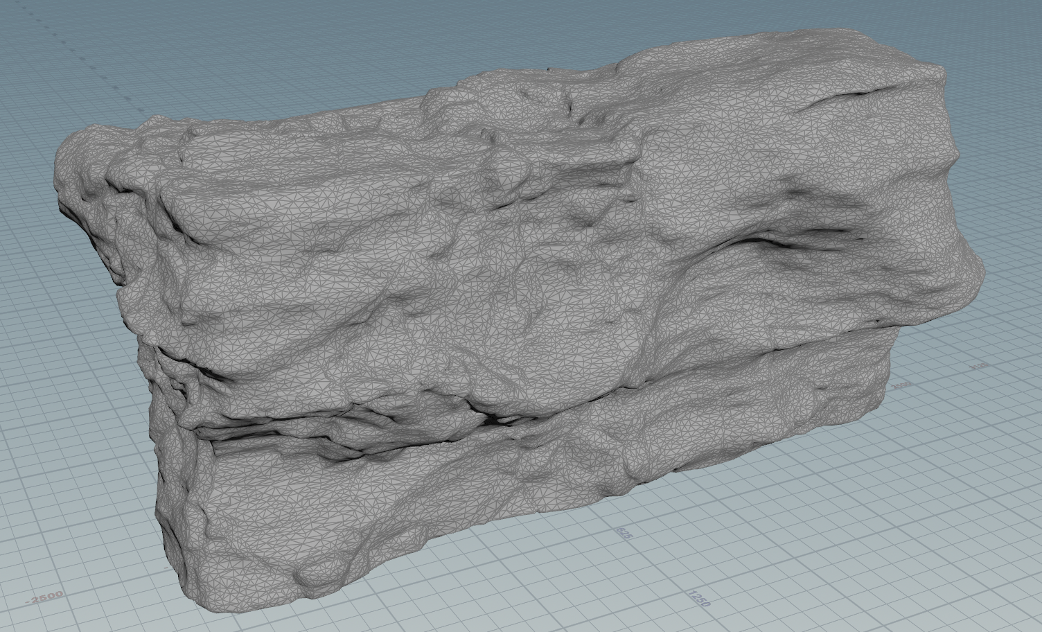
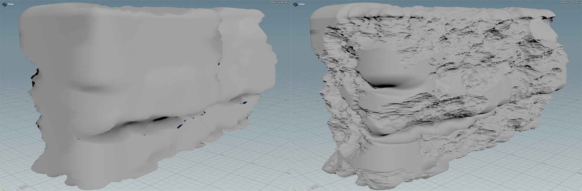
Here is a lower poly version of that cliff mesh that has 2 tiling displacement maps on it, that I will eventually mix with at least one more, and will paint them in and out in different places. But for now, both blending together at different resolutions:

From a ground level, I’m pretty happy with the results, with a bit of work on the displacement maps I think it could look decent!

The base mesh is very reasonable (around 90k Nanite triangles when imported into Unreal)!

At the very least this can be faster iteration, but depending on how much you can re-use displacement textures, it can also be a big disk space and maybe memory saving!

I could move more details into the base mesh given how well Nanite compresses.
But while Houdini has some great UV tools, but they are pretty slow on big meshes, don’t guarantee no overlaps, and I haven’t had a lot of luck fixing that with the various tools available (will try again at some point).

So keeping this low enough that I can manually mark seams works well for me personally:

A mesh this low only took me about 20 minutes to set up seams for, which is not bad at all, and then the subsequent unwrap was pretty clean due to the lower detail, and only takes a few seconds to run the actual unwrap itself.

Not a fair comparison, but that mesh ends up being less than 2Mbs with a bit of tuning Trim Relative Error (which is vastly faster to tune on a mesh this density)!

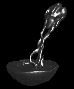
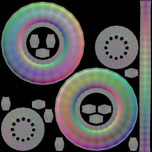
The displacement maps are pretty rough and generated out of Substance Designer using some of the base noises:

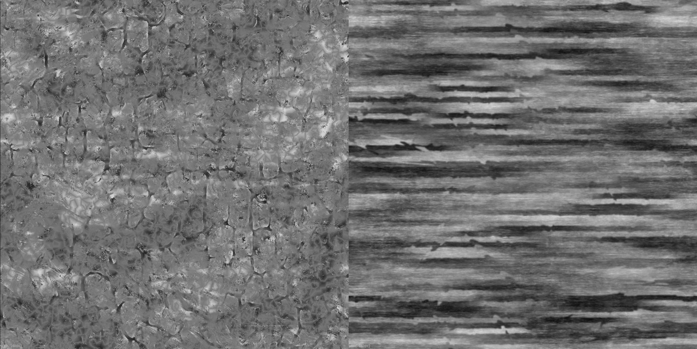
I also generated out normals and AO, which for the time being is necessary, I’ll go into that a bit.

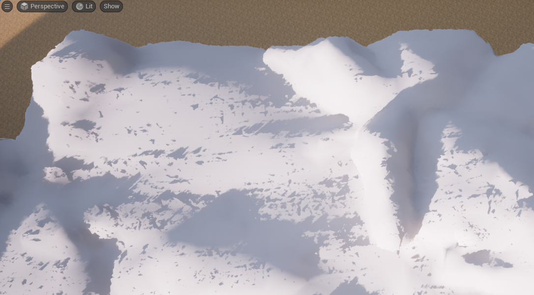
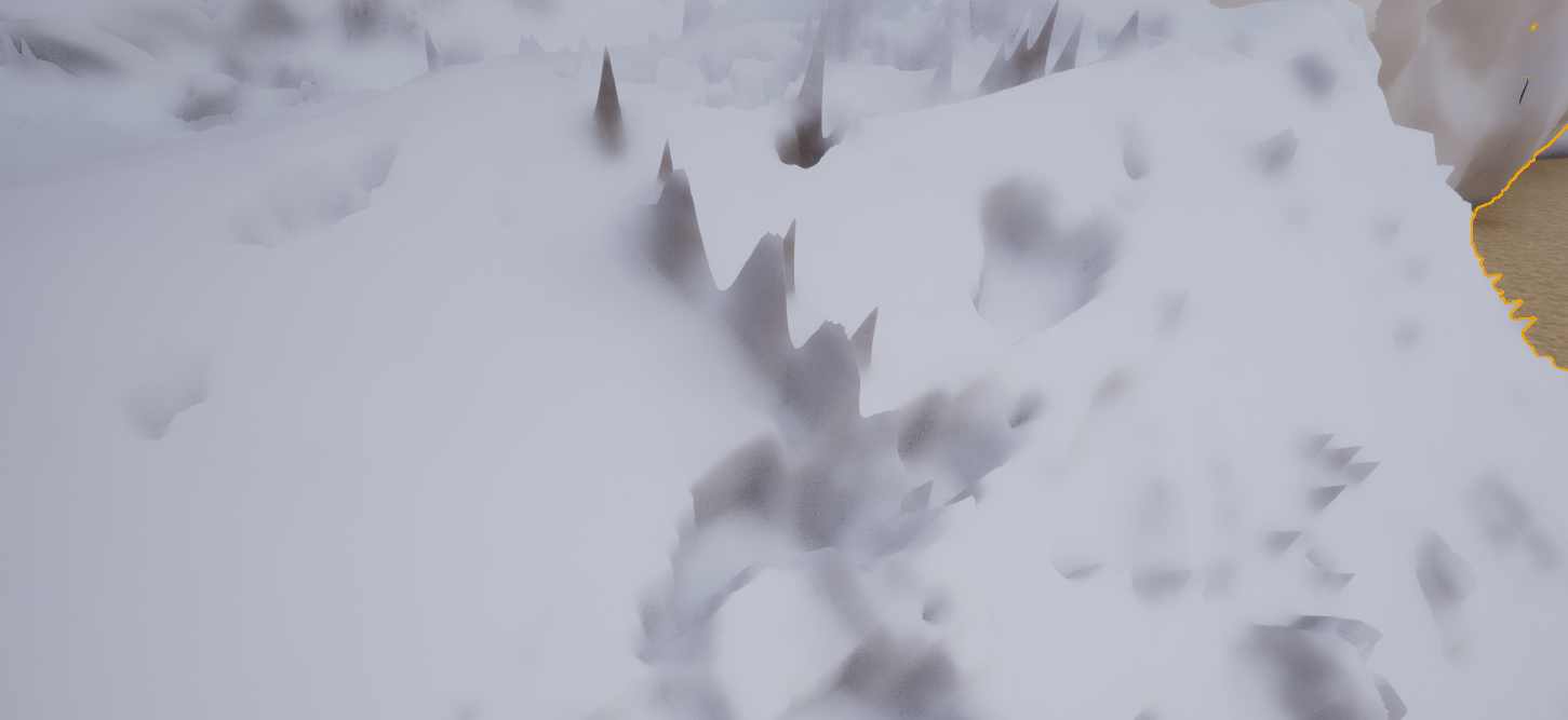
Initially when I turned on Nanite Tessellation I wasn’t sure it was working, because it looked like this:

But then it was obvious from the silhouette that it was working, so I wasn’t sure why I wasn’t seeing better details, and it took me a little while to work it out.

The shadows also showed it was doing *something* but it didn’t look quite right:

When you get close to the mesh, Lumen traces start giving you a bit more, and you start to see some detail, so that was another clue that it was definitely working (exaggerated displacement here):

And finally when you look at world normals it is obvious why:

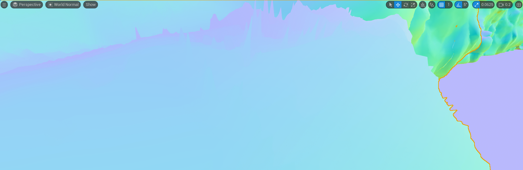
Nanite Tessellation doesn’t update normals (assuming I didn’t mess something up, which is a big assumption…)

I was a bit surprised by this at first, but probably shouldn’t have been, this is also true of Displacement in Houdini if you don’t manually update normals after doing it:

I’m hoping at some point in the future there might be a feature that does *something* with normals, but in the meantime I’d recommend always pairing displacement maps with normal maps.

The other issue you may have noticed in a few of the screenshots is meshes splitting at UV seams:

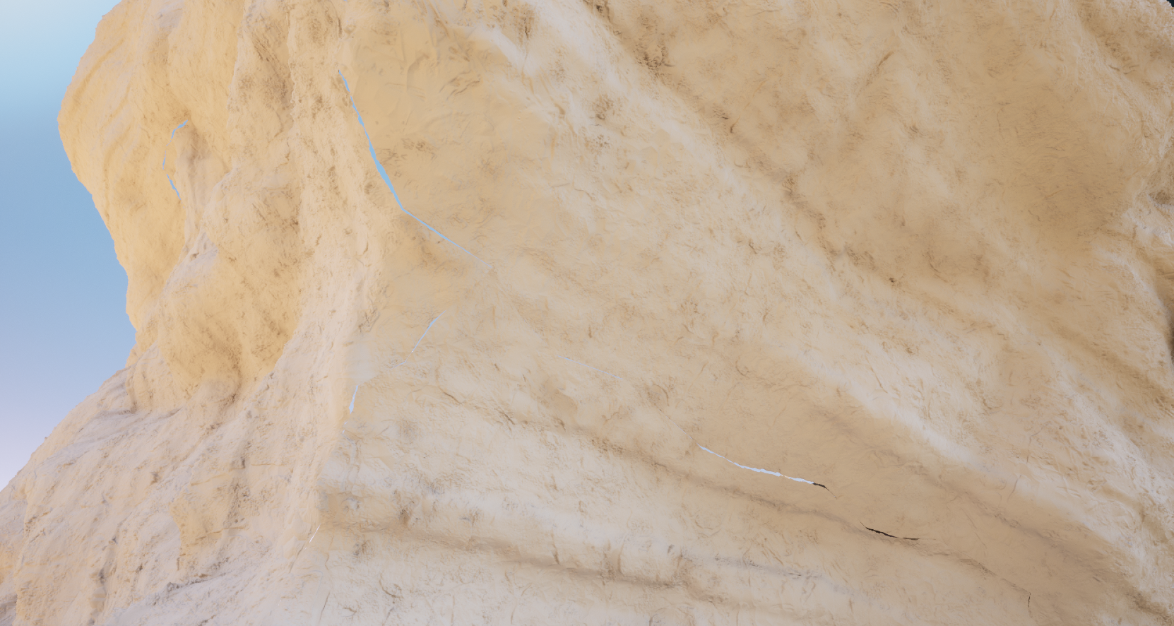
I think for this reason you’re likely to see Nanite Tessellation mostly used on ground planes, or walls, or anything that can feasibly unwrap in a single UV sheet for now.

But with some better unwrapping than I’ve done, maybe marking up seams with vertex colours in Houdini and then blending the displacement down around them with some sort of falloff, and then also augmenting with a bunch of smaller rock pieces would cover them up.

You may also be able to mitigate this by using projected textures more, assuming you can live with the cost and issues that come with tri-planar or whatever other approach.

Thoughts

Super impressed with Nanite Tessellation!
I probably should have spent more time with it before this post, but I was too excited to try it out and share my thoughts, please comment if I got anything horribly wrong or if you have your own thoughts on some of my assumptions / comments!

I think it’s going to be a really big deal for a lot of teams, and potentially a massive production cost savings. Building a library of great tiling detail displacement maps could really speed up iteration for certain types of assets.

On top of that, I haven’t even started looking at options for animating them!
There is likely all sorts of very fun things you can do with animated displacement maps in Nanite, can’t wait to see what clever artists do with it 🙂

AI budget tool (a 2014 revisit)

Blast from the past

I originally drafted this blog post a year or so after Splinter Cell: Blacklist launched, and I was still at Ubisoft (around 2014)!

I decided to hold off publishing it since there weren’t any active Splinter Cell projects at the time, and I always figured I’d come back to it and hit publish at a later date.
And well… here we are, very exciting stuff to come from Ubisoft Toronto and their partner studios 🙂

I’ve left the blog post largely as I wrote it back then, and in hindsight it’s pretty funny to think that I was working in Unreal 2, on a game mode that was inspired by the Gears Of War Horde game modes, years before I made the move to The Coalition to work on Gears!

Extraction (Charlie’s Missions)

When working on Splinter Cell: Blacklist, we had guidelines for the numbers of AI spawned.

So a heavy AI might be worth 1.1 bananas, and a dog 0.7 bananas, with a total banana budget of 10. The numbers roughly mapped to CPU budgets in milliseconds, but the important thing really was the ratio of costs for the various archetypes.

It’s a tricky thing to manage AI budgets across all the game modes and maps, and probably something that the Design department and AI programmers lost lots of sleep over.

Where it got particular tricky was in the CO-OP Extraction game mode.

The game mode has “waves” (a round of AI that is finished only when all of the enemies have been dealt with).

Within waves there are sub-waves, where AI have various probabilities of spawning, and these sub-waves can start either based off numbers of take downs in a previous sub-wave, or based off time.

So the player, for example, could just happen to let the most computationally expensive enemies live in a sub-wave, take out all the computationally cheap enemies (with tactical knock out cuddles, of course), and the next sub-wave could spawn in and we’d blow our AI budgets!

The team building the co-op maps in our Shanghai studio were great at sticking to the budgets, but this variation in the spawning for AIs was obviously going to be very hard to manage.

Having our QC team just test over and over again to see if the budgets were getting blown was obviously not going to be very helpful.

XML and C#/WPF to the rescue

Luckily, one of the engineers who was focused on Extraction, Thuan Ta, put all of the Extraction data in XML. This is not the default setup for data in the Unreal engine, almost all of the source data is in various other binary file formats, but his smart choice saved us a lot of pain.

It made it incredibly easy for me to spend a week(ish) bashing together this glorious beast:

A feat of engineering and icon design, I hear you say!!
Certainly can never be enough Comic Sans in modern UI design, in my opinion…

What is this I don’t even

Each row is an AI wave that contains boxes that represent varying numbers of sub-waves.

The sub-wave boxes contain an icon for each of the different AI types it might spawn, assuming the worst case (most expensive random AI) for that sub-wave (heavy, dog, tech, sniper, regular with a helmet, etc):

The number at the top right of each sub-wave box is the worst case AI cost that can occur in that sub-wave, and it can be affected by enemy units that carry over from the previous sub-wave:

So, for example, if sub-wave 1 has a chance of spawning 0-2 heavies, and 1-3 regulars, but only to a max number of 4 enemies, the tool will assume 2 heavies get spawned (because they are more expensive), and 2 regulars get spawned to estimate the worst cost AI for the sub-wave.

If sub-wave 2 then has a trigger condition of “start sub-wave 2 when 1 enemy in sub-wave 1 is taken out” (killed, or convinced to calmly step away and consider their path in life), then the tool would assume that the player chose to remove a regular in sub-wave 1, not a heavy, because regulars are cheaper than heavies.

Following this logic, the cost of each sub-wave is always calculated on the worst cases all the way to the end of the wave.

Long lived

Sometimes you’d want to know, at a glance, which enemies in a sub-wave can live on to the next sub-wave.

If you mouse over the header part of a sub-wave (where the orange circle is below), all the units that are created in that sub-wave are highlighted red, and stay highlighted in the following waves indicating the longest they can survive based off the trigger conditions for the following sub-waves:

So in the above case, the heavies that spawn in Wave 15, Sub-wave 1 can survive all the way through to sub-wave 3.

This is important, because if sub-wave 3 was over budget, one possible solution would be to change the condition on sub-wave 2 to require the player to take out one additional unit.

Also worth pointing out, the colour on the sub-wave bar headers are an indication of how close to breaking the budget we are, with red being bad. Green, or that yucky browny green are fine.
The colour on the bar on the far left (on the wave itself) is representative of the highest cost of any sub-wave belonging to this wave.
So you can see at a glance if any wave is over budget, and then scroll the list box over to find which sub-wave(s) are the culprits.

Listboxes of listboxes of listboxes

There’s about 300 lines of XAML UI for this thing, and most of it is a set of DataTemplates that set up the three nested listboxes: One containing all the waves, a listbox in each wave for the subwaves, a listbox in each sub-wave for the AI icons.

Each of the icon blocks has its own DataTemplate, which just made it easier for me to overlay helmets and shields onto the images for the different AI variants:

<datatemplate x:key="EAIShieldedHeavyController_Template" datatype="{x:Type local:Enemy}">
	<grid>
		<rectangle fill="Black" width="30" height="30" tooltip="Heavy + Shield">
			<rectangle.opacitymask>
				<imagebrush imagesource="pack://application:,,,/Icons/Heavy.png">
			</imagebrush></rectangle.opacitymask>
		</rectangle>
		<rectangle horizontalalignment="Right" verticalalignment="Bottom" fill="Green" width="15" height="15">
			<rectangle.opacitymask>
				<imagebrush imagesource="pack://application:,,,/Icons/Shield.png">
			</imagebrush></rectangle.opacitymask>
		</rectangle>
	</grid>
</datatemplate>

System.Xml.Linq.Awesome

Probably goes without saying, but even in a horrible hard-codey, potentially exception ridden hacky way like the way I was using it in this application, using the XDocument functionality in Linq makes life really easy 🙂

I definitely prefer it to XPath, etc.

Forgive me for one line Linq query without error handling, but sometimes you’ve got to live on the wild side, you know?:

_NPCTemplates = SourceDirInfo.GetFiles("*.ntmp").Select(CurrentFile => XDocument.Load(CurrentFile.FullName)).ToList();

And with those files, pulling out data (again, with error/exception handling stripped out):

foreach (XDocument Current in _NPCTemplates)
{
	// Get a list of valid NPC names
	foreach (XElement CurrentNPC in Current.Descendants("npc"))
	{
		List NameAttr = CurrentNPC.Attributes("name").ToList();
		if (NameAttr != null)
		{
			// Do things!!
		}
	}
}

Conclusion

Although it’s nothing particularly fancy, I really do like it when programmers choose XML for source data 🙂

It makes life really really easy for Tech Art folk, along with frameworks like WPF that really minimize the plumbing work you have to do between your data models and view, as well as making very custom (ugly) interfaces possible using composition in XAML.

Beats trying to create custom combo boxes in DataGrids in Borland C++ at any rate 😛

Also, Comic Sans. It’s the future.

Houdini looping particles

For a while I’d been planning to look into making looping particle systems in Houdini, but hadn’t found a good excuse to jump in. I don’t really do much VFX related work at the best of times, something I need to do more of in the future 🙂

Anyway, I was recently chatting with Martin Kepplinger, who is working on Clans Of Reign, and he was looking to do a similar thing!

So begins the looping particle journey…

Technique overview

I won’t go into the fluid sim setup, it doesn’t really matter too much what it is.

There are a few conditions that make my approach work:

• Particles must have a fixed lifetime
• The first chosen frame of the simulation must have a lead up number of frames >= the particle lifetime
• The last frame of the loop must be >= the first frame number + the particle lifetime

I have some ideas about how to get rid of these requirements, but not sure if I’ll get back to that any time soon.

For the example in this post, I am keeping particle lifetime pretty low (0.8 to 1.0 seconds, using a @life attribute on the source particles, so a 24 frame loop).

The fluid sim I’m using is some lumpy fluid going into a bowl:

The simulation is 400 frames long (not all shown here), but that ended up being overkill, I could have got away with a much shorter sim.

Going back to my rules, with particles that live 24 frames I must choose a first frame >= 24 (for this example, I’ll choose 44).
The last frame needs to be after frame 68, so I’m choosing 90.
This makes a loop that is 46 frames long, here it is with no blending:

The technique I’m going to use to improve the looping is somewhat like a crossfade.

For this loop from 44 –> 90, I’m modifying the particles in two ways:

1. Deleting any particles that are spawning after frame 66 (i.e, making sure all particles have died before frame 90)
2. From frames 66 to 90, copying in all the particles that spawn between frame 20 –> 44.

This guarantees that all the particles that are alive on frame 89 match exactly with frame 44.

To illustrate, this gif shows the unedited loop on the left, and next to it on the right is the loop with no new particles spawned after frame 66 (particles go red on 66):

Next up is the loop unedited on the left, and on the right are the new particles from frames 20 – 44 that I’m merging in from frame 66 onward:

And now, the unedited loop next to the previous red, green and blue particles combined:

And finally, just the result of the looping by itself without the point colours:

One thing that might be slightly confusing about the 2nd gif with the green pre-loop particles is that I’m always spawning particles in the bowl itself to keep the fluid level up, in case you were wondering what that was about 🙂

Setting up the loop

This is the SOPs network that takes the points of a particle sim, and makes it loop:

The first part of setting up the looping simulation is picking the start and end frames (first and last) of the loop.

I created a subnetwork (FrameFinder, near the top of the above screenshot) that has parameters for two frame numbers, and displays a preview of the two frames you are selecting, so you can find good candidates for looping:

The loop setup I chose for the Unity test at the top of the blog was actually a bit different to the range I chose for the breakdowns in the last section.
For Unity, I wanted the shortest looping segment I could, because I didn’t want it to be super expensive (memory wise), so I chose start and end frames 25 frames apart.

You can see that the frames don’t need to match exactly. The main thing I wanted to avoid was having a huge splash in the bowl at the bottom, or over the edge, because that would be hard to make look good in a short loop.

Node parameters

In the screenshot above, you can see that I have First Frame and Last Frame parameters on my FrameFinder network.

I don’t tend to make my blog posts very tutorial-y, but I thought I’d just take the time to mention that you can put parameters on any node in Houdini.

Example:

• Drop a subnetwork node
• Right click and select “Parameters and Channels –> Edit Parameter Interface…”:
• Select a parameter type from the left panel, click the arrow to add the parameter, and set defaults and the parameter name on the right:
• Voila! Happy new parameter:
  

You can then right click on the parameter and copy a reference to it, then use the reference in nodes in the subnetwork, etc.
In the edit parameter interface window, you can also create parameters “From Nodes”, which lets you pick an existing parameter of any node in the sub network to “bubble up” to the top, and it will hook up the references.

If this is new to you, I’d recommend looking up tutorials on Digital Assets (called “HDAs”, used to be called “OTLs”).

I do this all the time on subnetworks like on the FrameFinder, but also to add new fields to a node that contain parts of an expression that would get too big, or that I want to reference from other nodes, etc.

On Wrangles (for example), I find myself adding colour ramp parameters a lot for use within the wrangle code.

FrameFinder

This subnetwork has two outputs: the particles with some Detail Attributes set up, and another output that is a preview of the two frames which I showed before, but here’s what that looks like again:

It’s the first time I’ve created multiple outputs from a subnetwork, usually I just dump a “Preview” checkbox as a parameter on the network, but I like this more I think, particularly if I end up turning the whole thing into an HDA.

Here is what the FrameFinder network looks like:

In this project, I’m using Detail attributes to pass around a lot of data, and that starts in with the attribcreate_firstAndLastFrame node.

This node creates Detail parameters for each of the frames I chose in the subnet parameters (firstFrame and lastFrame):

Right under the attribCreate node, I’m using two timeshift nodes: one that shifts the simulation to the first chosen frame, and one to the last frame, and then I merge them together (for the preview output). I’ve grouped the lastFrame particles so that I can transform them off to the right to show them side by side, and also giving all the particles in both frames random colours, so it’s a little easier to see their shape.

Time ranges and ages

Back in the main network, straight after the frameFinder subnetwork I have another subnetwork called timeRangesAndAges, which is where I set up all the other Detail attributes I need, here is what is in that subnetwork:

The nodes in the network box on the right side are used to get the maximum age of any particle in the simulation.
In hindsight, this is rather redundant since I set the max age on the sim myself (you could replace all those nodes with an Attribute Create that makes a maxAge attribute with a value of 24), but I had planned to use it on simulations where particles are killed through interactions, etc 🙂

The first part of that is a solver that works out the max age of any particle in the simulation:

For the current frame of particles, it promotes Age from Point to Detail, using Maximum as the promotion method, giving me the maximum age for the current frame.

The solver merges in the previous frame, and then uses an attribute wrangle to get the maximum of the previous frame and current frame value:

@maxAge = max(@maxAge, @opinput1_maxAge);

Right after the solver, I’m timeshifting to the last frame, forcing the solver to run through the entire simulation so that the MaxAge attribute now contains the maximum age of any particle in the simulation (spolier: it’s 24 :P).

I then delete all the points, since all I care about is the detail attribute, and use a Stash node to cache that into the scene. With the points deleted, the node data is < 12 Kb, so the stash is just a convenient way to stop the maxAge recalculating all the time.
If I turn this whole thing into an HDA, I’ll have to rethink that (put “calculate max particle age” behind a button or something).

There are two more wrangle nodes in time ranges and ages.

One of them is a Point wrangle that converts the particle age from seconds into number of frames:

@frameAge = floor(@age/@TimeInc);

And the next is a Detail wrangle that sets up the rest of the detail attributes I use:

// Copy max age from input 1
int maxAge = i@opinput1_maxAge;

// A bunch of helper detail variables referenced later
int loopLength = i@lastFrame - i@firstFrame;
int loopedFrame = (int)(@Frame-1) % (loopLength+1);

i@remappedFrame = i@firstFrame + loopedFrame;

int distanceFromSwap = loopedFrame - loopLength;

i@blendToFrame = max(1, i@remappedFrame - loopLength);
i@numberOfFramesIntoBlend = max(0, maxAge + distanceFromSwap);

When I hit play in the viewport, I want to see just the looping segment of the simulation over and over, so that complicates all this a little.

With that in mind, there are 3 important attributes set up here.

@remappedFrame

If my start frame is 20, for example, and the end frame is 60, I want to see the 20-60 frame segment over and over, hence the wrapping loopedFrame temporary variable.

So if my viewport time slider is on 15, I really want to see frame 34, the value of remappedFrame will be 34. It will always be a number between firstFrame and lastFrame.

@blendToFrame

This takes the remappedFrame, and shifts it back to before the start of the loop.
I only use this value when we hit the last 24 frames of the loop, but I’m clamping it at one just so the timeshift I use later doesn’t freak out.

This attribute will be used in the 2nd part of the technique: combining in pre-loop particles.

@numberOfFramesIntoBlend

When we are getting into the last 24 frames of the loop, this value increases from 0 to 24.
It’s used in the 1st part of the technique to stop spawning particles that have an age less than this value.

Timeshifts and recombining particles

Back to the main network:

After the timeRangesAndAges node, the network splits: on the left side, I’m timeshifting the simulation using the remappedFrame detail attribute as the frame using this expression:

detail("../timeRangesAndAges/", "remappedFrame", 0)

On the right side I’m time shifting the simulation using the blendToFrame attribute as the frame using this expression:

detail("../timeRangesAndAges/attribwrangle_calcTimeRanges", "blendToFrame", 0)

I’ve colour coded the nodes in the network with the same colours I’ve shown in the gifs in the technique section.

Since I’ve timeshifted the simulation, the detail attributes get time-shifted too.
But I don’t really want that, so I’m attribute transferring the two detail attributes I care about (remappedFrame and numberOfFramesIntoBlend) back onto the remapped sims using Attribute Transfer.

After the attribute transfers, on both sides I’m creating a new point group called inBlendingFrames.

detail(0, "numberOfFramesIntoBlend", 0) > 0

I probably didn’t need a point group for this, considering every particle is either in or out of this group on a given frame, it just made life easier with the Split node I use on the left.

On the left side, I do a split using inBlendingFrames.
When we’re not in the blending range, we don’t have to do anything to the particles, so that’s the blue colour node.

For both the red and green nodes section, I start with deleting anything not in the inBlendingFrames group.

For the green particles (the pre-loop particles that we’re merging in), we’ve already got the right frame, due to the timeshift up the top.
If we’re on blending frame 2 of the blend (for example), we will still have particles that were spawned 24 frames ago, but we really only want particles that should spawn after the blend starts.
I use an attribute wrangle to clean the older particles up, since I have the frameAge attribute I can use:

if ((@frameAge > i@numberOfFramesIntoBlend))
{
	removepoint(0, @ptnum);
}

Here’s what that looks like for a frame about halfway through the blend.

For the red nodes section (where we take the original loop, and delete any particles that start spawning after the blend), I use an attribute wrangle to clean the new particles up:

if (@frameAge < i@numberOfFramesIntoBlend)
{
	removepoint(0, @ptnum);
}

So, I merge the red, blue and green particles all together, and we end up with the result I showed in the technique section!

Here again uncolourised:

Unity, Alembic and all that jazz

This post is already crazy long, so I’m just going to gloss over the Houdini –> Unity stuff.
If anyone is really interested in those details, I might do another post.

So now that I have a looping particle system, I can use a regular Particle Fluid Surface with default settings, and a polyreduce node to keep the complexity down:

I exported the range of frames as an Alembic file, and imported it into Unity with the Alembic plugin.

I threw together a really quick monoBehaviour to play the Alembic stream:

using System.Collections;
using System.Collections.Generic;
using UnityEngine;
using UTJ.Alembic;

[RequireComponent(typeof(AlembicStreamPlayer))]
public class PlayAlembic : MonoBehaviour
{
	public float playSpeed = 0.02f;

	AlembicStreamPlayer sPlayer;

	// Use this for initialization
	void Start ()
	{
		sPlayer = GetComponent();
	}

	// Update is called once per frame
	void Update () 
	{
		sPlayer.currentTime += playSpeed;
		sPlayer.currentTime = sPlayer.currentTime % 1.0f;
	}
}

As a last little thing, I packaged the network up a lot neater, and dumped it in a loop that ran the process on 16 different 46 frame range segments of the original simulation.
The idea being, why try to find good first and last frames when you can just go for a coffee, and come back and have 16 to choose from!

The loops with big splashes definitely don’t work very well (they look like they aren’t looping because lots of particles dying on the same frame), but there are some fun examples in here:

Faking Catmull-Clark creased sub-d in UE4

I’ve been hoping for edge creased Catmull-Clark subdivision in game engines ever since I started using Modo about 10 years ago.
I previously made a tool to build LODs from sub-d surfaces in Unity, just to have some way of getting a sub-d like mesh in engine. Super expensive LOD meshes…
This was not a very useful thing to do.

There are a few games out there using real-time sub-d, including the folks at Activision who have demonstrated CC sub-d with creases in a game engine:

Efficient GPU Rendering of Subdivision Surfaces using Adaptive Quadtrees

It is unclear if they shipped edge-creasing in any of their released games, but they definitely use CC subdivision surfaces.

And sure, technically there has been real-time subdivision in games going back to TruForm on ATI cards in the early 2000s, and probably before then for all I know, but I’m specifically interested in Catmull-Clark sub-d, and specifically edge creasing 🙂

Why creases?

Creasing gives you control over the sharpness of edges, without having to manually bevel all of your edge loops.
This is nice for keeping a low poly mesh, but also allows you a little more flexibility.
For example, if you come back and change the model, you don’t have to un bevel and re-bevel edges.
If you bake out a normal map, and decide the bevels aren’t quite wide enough, you can just change the crease value and re-bake.

Here are some loops on my wheel model that are heavily creased:

If I were to bevel those edges instead, my base model would go from 3924 vertices to 4392.

If I removed creases across the whole model, and beveled all the edges to get the same end result I’d need a base mesh around 6000 vertices (2000 vertices more than the creased version).

For the sake of showing how much work the creasing is doing for me, here is the base model vs Sub-d vs Creased Sub-d:

Vector Displacement approach

I’m not likely to be able to implement the Call Of Duty approach myself, so I’ve done something far more hacky, but slightly less gross than my previous Unity attempt 🙂

My new method is:

• In Houdini, tessellate the model completely flat
• Also tessellate it using Catmull Clark creased sub-d
• Bake the difference in positions of the vertices between these two meshes into a vector displacement map and normal map
• In UE4 (or engine of choice) flat tessellate the model
• Apply the vector displacement map to push the vertices into their sub-d positions

It’s very expensive from a memory point of view (and probably performance for that matter), so this is not something you’d want to do for a game, but it does show off how nice creased sub-d would be in UE4 🙂

Houdini Vector displacement map generation

First up, here’s the un-subdivided model in Modo:

And this is the edge weighting view mode in Modo, so you can see which edges are being creased:

There are two things I want to bake out of Houdini: A vector displacement map and a normal map.
I’m not baking this data by projecting a high poly model onto a low poly, I don’t need to because the high poly model is generated from the low poly, so it has valid UVs, I can just bake textures straight out from the high poly.

Here’s the main network:

The right side of the graph, there are two Subdivide nodes.
The Subdivide on the left uses “OpenSubdiv Blinear”, and on the right is “OpenSubdiv Catmull-Clark”, and they are both subdivided to a level of 5, so that I have roughly more vertices in the meshes than pixels that will get baked out:

The “bilinear” subdivision is pretty close to what you get in UE4 when you use “flat tessellation”. So what we want to do is work out how to push the vertices from the left model to match the right model.
This is very easily done in a Point Wrangle, since the point numbers match in both models 🙂

v@vDisp = @P - @opinput1_P;
@N = @opinput1_N;
f@maxDimen = max(abs(v@vDisp.x), abs(v@vDisp.y), abs(v@vDisp.z));

Or if you’d prefer, as a Point VOP:

Vector displacement (vDisp) is the flat model point position minus the creased model point position.
I am also setting the normals of the flat model to match the creased model.

When I save out the vector displacement, I want it in the 0-1 value range, just to make my life easier.
So in the above Wrangle/VOP I’m also working out for each Point what the largest dimension is (maxDimen).
After the Wrangle, I promote that to a Detail attribute (@globalMaxDimen) using the Max setting in the Attribute Promote SOP, so that I know the maximum displacement value across the model, then use another Wrangle to bring all displacement values into the 0-1 range:

v@vDisp = ((v@vDisp / f@globalMaxDimen) + 1) / 2;
@Cd = v@vDisp;

The displacement is now stored in Point colour, in the 0-1 range, and looks like this:

Bake it to the limit!.. surface

You might have noticed that the Normals and Displacement are in World space (since that’s the default for those attributes in Houdini).

I could have baked them out in Tangent space, but I decided for the sake of this test I’d rather not deal with tangent space in Houdini, but it’s worth mentioning since it’s something I need to handle later in UE4.

To bake the textures out, I’m using two Bake Texture nodes in a ROP network in Houdini.

I’ve only changed a few settings on the Bake Texture nodes:

• Using “UV Object”, and no cage or High Res objects for baking
• Turned on “Surface Unlit Base Color” as an output
• Set the output format for Vector Displacement as EXR
• Set the output format for Normal map as PNG
• Unwrap method to “UV Match” (since I’m not tracing from one surface to another)
• UDIM Post Process to Border Expansion

And what I end up with is these two textures:

I bake them out as 4k, but lodbias them down to 2k in UE4 because 4k is a bit silly.
Well, 2k is also silly, but the unwrap on my model is terrible so 2k it is!

Testing in Houdini

If you look back at the main network, there is a section on the left for testing:

I created this test part of the network before I jumped into UE4, so I could at least validate that the vector displacement map might give me the precision and resolution of data that I would need.
And also because it’s easier to debug dumb things I’ve done in a Houdini network vs a material in UE4 (I can see the values of every attribute on a vertex, for example) 🙂

I’m taking the flat tessellated model, loading the texture using attribvop_loadTexture, copying the globalMaxDimens onto the model, and then the attribwrangle_expectedResult does the vector displacement.

The attribvop_loadTexture is a Vertex VOP that looks like this:

This uses the Vertex UVs to look up the vector displacement map texture, and stores the displacement in vertex colour (@Cd). It also loads the object space normal map, and moves it from 0-1 to -1 to 1, and binds it to a temporary loadedNormals attribute (copied into @N later).

Then at the end of the network, the expectedResult wrangle displaces the position by the displacement vector in colour, using the globalMaxDimen:

@P -= ((@Cd * 2) - 1) * f@globalMaxDimen;

If you’re wondering why I’m doing the (0 –> 1) to (-1 –> 1) in this Wrangle, instead of in the VOP (where I did the same to the normal), it’s because it made me easier to put the reimportUvsTest switch in.
This (badly named) switch allows me to quickly swap between the tessellated model with the displacement values in vertex colour (before bake), and the tessellated model that has had that data reloaded from texture (after bake), so I can see where the texture related errors are:

There are some errors, and they are mostly around UV seams and very stretched polygons.
The differences are not severe enough to bother me, so I haven’t spent much time looking into what is causing it (bake errors, not enough precision, the sampling I’m using for the texture, etc).

That’s enough proof in Houdini that I should be able to get something working in engine, so onwards to UE4!

UE4 setup

In UE4, I import the textures, setting the Compression on the Vector Displacement Map to be VectorDisplacementmap(RGBA8), and turn off sRGB.
Yay, 21 Mb texture!

I can almost get away with this map being 1024*1024, but there is some seam splitting going on:

That might be also be solved through more aggressive texture Border Expansion when baking, though.

Here is what the material setup looks like (apologies for the rather crappy Photoshop stitching job on the screenshots, but you can click on the image to see the details larger):

The value for the DisplaceHeight parameter is the @globalMaxDimen that I worked out in Houdini.

Since both textures are Local (Object) space, I need to shift them into the right range (from 0-1 to -1 to 1), then transform them into World space (i.e, take into account the objects rotation and scale in the scene, etc).

The Transform node works fine for converting local to world for the Normal map.
I also needed to set the material to expect world space normals by unchecking Tangent Space Normal:

The Transform node works fine for normal maps, but does not work for things that are plugged into World Displacement.
Tessellation takes place in a hull / domain shader and the Local -> world transformation matrix is not a thing it has access to.
To solve this properly in code, I think you’d probably need to add the LocalToWorld matrix into the FMaterialTessellationParameters struct in MaterialTemplate.usf, and I imagine you’d need to make other changes for it to work in the material editor, or you could use a custom node to access the matrix.

If you look back at my material, you can see I didn’t do that: I’m constructing the LocalToWorld matrix from vectors passed in as material parameters.
Those parameters are set in the construction script for blueprint for the object:

I’m creating a dynamic material instance of the material that is on the object, applying this new instance to the object, and setting the Up, Right and Forward vector parameters from the Actor. These vectors are used in the material to build the local to world space matrix.

If I wanted the object to be animated, I’d either need to do the proper engine fix, or do something nasty like update those parameters in blueprint tick 🙂

Results in UE4

Please ignore the albedo texture stretching, I painted it on a medium divided high poly mesh in Substance Painter, probably should have used the low poly (something for me to play with more at a later date).

This is with a directional light and a point light without shadows.
As a side note, Point Light shadows don’t seem to work at all with tessellated objects in UE4.

Spotlight and directional light shadows work ok, with a bit of a caveat.
They use the same tessellated mesh that is used for the other render passes, so if the object is off screen, the shadows will look blocky (i.e, it seems like tessellation is not run again in the shadow pass from the view of the light, which probably makes sense from an optimization point of view):

And that’s about it!

Seems like a lot of work for something that is not super useful, but it’s better than my last attempt, and being built in Houdini it would be very easy to turn this into a pipeline tool.

For lots of reasons, I’m skeptical if I’ll ever work on a project that has Catmull-Clark creased sub-d, but at least I have a slightly better way of playing around with it now 🙂

 

 

 

 

 

Chopped Squabs – Pt 4

 

Last post was about smoke, particles and weird looking ball things.
This post is about the audio for the video.

I wanted to make a sort of windy / underwater muffled sound, and managed to get somewhat close to what I wanted, just using Houdini CHOPs!

Pulse Noise

I decided not to create the audio in the same hip file, since it was already getting a bit busy, and because the data I want to use is already cached out to disk (geometry, pyro sim, etc).

The new hip file just has a small geometry network and a chops network.
Here’s the geometry network:

I wanted the audio to peak at times where the pulse was peaking on the tuber bulbs, so the first step was to import the bulbs geometry:

Next I’m promoting the pulse amount from points to detail, using “sum” as the promotion method (this adds up all the pulse amounts for all points in the bulbs every frame).
I don’t care about the geometry any more, because the sum is a detail attribute, so I delete everything except for a single point.

I had a bit of a hard time working out how to bring the values of a detail attribute into CHOPs as a channel. I think it should be simple to do with a Channel CHOP, but I didn’t succeed at the magic guessing game of syntax for making that work.

Anyway, since importing point positions is easy, I just used an attribute wrangle to copy the pulse sum into the position of my single point:

@P = detail(@opinput1, "pulse");

Audio synthesis fun

I had some idea of what I wanted, and how to make it work, from experiments in other software (Supercollider, PureData, etc).

I found that creating an interesting wind sound could be achieved through feeding noise into a lowpass filter.

I also tried this out in Unity, grabbing the first C# code I could find for filters:
https://stackoverflow.com/questions/8079526/lowpass-and-high-pass-filter-in-c-sharp

Here is a Unity MonoBehaviour I built from that code above:

using System;
using System.Collections;
using System.Collections.Generic;
using UnityEngine;

[RequireComponent(typeof(AudioSource))]
public class PlayerAudio : MonoBehaviour
{
    AudioSource _requiredAudioSource;
    public int _samplerate = 44100;

    private const float _resonance      = 1.0f;
    private float _phase                = 0.0f;
    private float _rampInAmount         = 0.0f;
    private float _frequency            = 800.0f;
    private System.Random _rand1        = new System.Random();
    private float[] _inputHistory       = new float[2];
    private float[] _outputHistory      = new float[3];

    void Start ()
    {
        _requiredAudioSource = GetComponent<AudioSource>();
        AudioClip testClip = AudioClip.Create("Wind", _samplerate * 2, 1, _samplerate, true, OnAudioRead);
        _requiredAudioSource.clip = testClip;
        _requiredAudioSource.loop = true;
        _requiredAudioSource.Play();
    }

    void Update ()
    {
        _rampInAmount = Mathf.Min(_rampInAmount + (Time.deltaTime/2.0f), 1.0f);
    }

    void OnAudioRead(float[] data)
    {
        float c, a1, a2, a3, b1, b2;

        for (int i = 0; i < data.Length; i++)
        {
            // Create a random amplitude value
            double currentRand  = _rand1.NextDouble();
            float amplitudeRand = (float)(currentRand * 2.0f - 1.0f) * _rampInAmount;
            amplitudeRand /= 2.0f;

            // Phase over a few seconds, phase goes from 0 - 2PI, so wrap the value
            float randRange = Mathf.Lerp(-1.0f, 1.0f, (float)currentRand);
            _phase += 1.0f / _samplerate;
            _phase += randRange * 200.0f / _samplerate;
            _phase %= (Mathf.PI * 2.0f);

            float interpolator = (Mathf.Sin(_phase) + 1.0f) / 2.0f;
            _frequency = Mathf.Lerp(100, 200, interpolator);

            // Low pass filter
            c = 1.0f / (float)Math.Tan(Math.PI * _frequency / _samplerate);
            a1 = 1.0f / (1.0f + _resonance * c + c * c);
            a2 = 2f * a1;
            a3 = a1;
            b1 = 2.0f * (1.0f - c * c) * a1;
            b2 = (1.0f - _resonance * c + c * c) * a1;

            float newOutput = a1 * amplitudeRand + a2 * this._inputHistory[0] + a3 * this._inputHistory[1] - b1 * this._outputHistory[0] - b2 * this._outputHistory[1];

            this._inputHistory[1] = this._inputHistory[0];
            this._inputHistory[0] = amplitudeRand;

            this._outputHistory[2] = this._outputHistory[1];
            this._outputHistory[1] = this._outputHistory[0];
            this._outputHistory[0] = newOutput;

            data[i] = newOutput;
        }
    }
}

It’s pretty gross, doesn’t work in webgl, and is probably very expensive.
But if you’re a Unity user it might be fun to throw in a project to check it out 🙂
I take no responsibility for exploded speakers / headphones…

With that running, you can mess with the stereo pan and pitch on the Audio Source, for countless hours of entertainment.

Back to Chops

When testing out Audio in a hip file, I could only get it to play if I use the “Scrub” tab in the audio panel.
You need to point it to a chopnet, and make sure that the chopnet is exporting at least one channel:

You should also make sure that the values you output are clamped between -1 and 1, otherwise you’ll get audio popping nastiness.

The CHOP network I’m using to generate the audio looks like this:

What I’d set up in Unity was a channel of noise that is run through a High Pass filter with a varying Cutoff amount.
I tried to do exactly the same thing in Houdini: Created a noise chop, a Pass Filter chop, and in the Cutoff field sample the value of the noise chop using an expression:

chop("chan1")

I was hoping that the whole waveform would be modified so I could visualize the results in Motion FX View, but what I found instead is that the waveform was modified by the current frames noise value in Motion FX.
With my limited knowledge of CHOPs, it’s hard to describe what I mean by that, so here’s gif of scrubbing frames:

It’s likely that it would still have given me the result I wanted, but having the wave form jump around like that, and not being able to properly visualize it was pretty annoying.

So, instead of creating noise to vary the high pass cutoff, I instead created a bunch of noise channels, and gave each of them their own high pass cutoff, then I blend those together (more on that part later).

In my Pass Filter, I created two new parameters (using Edit Parameter Interface) that I refence from a few different nodes:

Through trial and error, I found that low cutoff values from 0.3 to 0.6 gave me what I want, so I use an expression to filter each of the channels with a cutoff in that range, based on the channel ID:

ch("baseCutoff") + (fit($C/(ch("passBands")-1), 0, 1, 0.2, 0.5))

The baseCutoff is sort of redundant, it could just be built into the “fit” range, but I was previously using it in other nodes too, and never got around to removing it 🙂

I’m using the “passBands” parameter in that expression, but I also use it in the Channel creation in the noise CHOP:

It probably would have been more sensible just to hard code the number of channels here, and then just count how many channels I have further downstream, but this works fine 🙂

In the Transform tab of the noise, I’m using $C in the X component of the Translate, to offset the noise patterns, so each channel is a bit different. In hindsight, using $C in the “seed” gives a better result.

So now I have some channels of filtered noise!
I’ll keep passBands to 5 for the rest of this post, to keep it easy to visualize:

Combining noise and pulse

The top right part of the CHOP network is importing the pulse value that I set up earlier.

I’m importing a single point, and the pulse value was copied into Position, as mentioned earlier.
I’m deleting the Y and Z channels, since they are the same as X, normalizing the data using Limit, moving the data into the 0-1 range, and then lagging and filtering to soften out the data a bit.

Here is what the pulse looks like before and after the smoothing:

So this pulse channel is tx0, and I merge that in with all the noise channels (chan1-x).

I want to use the value of this pulse channel to blend in the noise channels I previously created.
So, for example, if I have 4 bands: between 0 and 0.25 pulse value I want to use band 1 noise, between 0.25 and 0.5 I’ll use band 2, 0.5 and 0.75 use band 3, etc.

I didn’t want a hard step between bands, so I’m overlapping them, and in the end I found that having quite a wide blend worked well (I’m always getting a little of all noise channels, with one channel dominant).

This all happens in the vopchop_combineNoiseAndPulse:

The left side of the network is working out the band midpoint ((1 / number of channels) * 0.5 * current channel number).

The middle section gets the current pulse value, and finds how far away that value is from the band midpoint for each channel.

If I just output the value of that fit node, and reduce the overlap, hopefully you can see what this is doing a little more obviously:

As the red line increases, it goes through the midpoints of each noise band, and the corresponding noise channel increases in intensity.

Since I’ve lowered the overlap for this image, there are actually gaps between bands, so there are certain values of the pulse that will result in no noise at all, but that’s just to make the image clearer.

The rest of the network is multiplying the pulse value with the noise channel value, and I end up with this:

With that done, I delete the pulse channel, and I add all the noise channels together.

The last thing I’m doing is outputting the noise in stereo, and for that I’m just arbitrarily panning the sound between two channels using noise.

I create two new stereo noise channels together, and then use a vop to flip the second channel:

So I end up with this:

I multiply this back on the original noise:

There’s a few other little adjustments in there, like making sure the amplitude is between -1 and 1, etc.

Also, I ramp in and out the audio over the first and last 20 frames:

And that’s it!

Hopefully you’ve enjoyed this series breaking down the squab video and my adventures in CHOPs. I can’t imagine I’ll use it for audio again, but it was definitely a fun experiment.

Today is Houdini 17 release day, so I can’t wait to dig in, and play around with all the new interesting features, perhaps there will be some vellum sims for future blog posts 🙂

Chopped Squabs – Pt 3

 

Last post, I talked about the tubers, their animation and creation of the pulse attributes.
This post will be about the bulbs on the end of the tubers, the pyro and particles setup.

Great balls of pyro

Since you don’t really get a close look at the tuber bulbs, considering the lighting and pyro cover them quite a bit, all of the bulbs have the same geometry.

Here is what the network looks like:

This is a rather silly thing to do procedurally, I should have just sculpted something for it. Because problem solving in Houdini is fun, I tend to do everything in my home projects procedurally, but there are definitely times where that is a) overkill and b) ends up with a worse result.

Anyway, I’m starting out with a sphere:

• Jittering the points a bit
• Extruding the faces (to inset them)
• Shrinking the extruded faces using the Primitive SOP on the group created by the extrude
• Extruding again
• Subdividing

That gives me this:

I’m then boolean-ing a torus on one side, which will be where the tuber connects to the bulb.
I didn’t really need to Boolean that, since just merging the two objects and then converting to VDB and back gives me pretty much the same result, which is this:

Then I remesh it, and apply some noise in an Attribute VOP using the Displace Along Normal.

Before the Attribute VOP, I’ve set up a “pores” attribute, which is set to 1 on the extruded inside faces, and 0 everywhere else.
The VOP adds some breakup to the pores attribute, which is eventually used for emissive glow:

There was a very scientific process here of “add noise nodes until you get sick of looking at it”.

Here is the result:

Looks ok if you don’t put much light on it, and you cover it with smoke 🙂

Spores / smoke

I wanted the smoke to look like a cloud of spores, sort of like a fungus sort of thing, with some larger spores created as particles that glow a bit.

The source of the smoke is geometry that has a non zero “pulse” attribute (that I set up in earlier posts), but I also just add a little bit of density from the pores on the tuber bulbs all the time.

So on any given frame I’m converting the following geometry to a smoke source:

The resulting smoke source looks like this:

I also copy some metaballs onto points scattered on this geometry, which I’m using in a to push the smoke around:

I’m feeding that metaball geometry into the magnet force in a SOP Geometry node:

I’m not going to break down the dynamics network much, it is mostly setup with shelf tools and minimal changes.

With the forces and collisions with tuber geometry, the smoke simulation looks like this:

Particles

The geometry for the tubers and bulbs is also used to create spawn points for emissive particles:

Kind of messy, but on the right I’m capping the tuber sections that I showed before, remeshing them by converting to vdb, smoothing then converting back to polygons, scattering some points, adding velocity and some identifying attributes.

On the left side, I’m scattering points on the bulbs when the density (pulse value) is high.

In both cases, I’m setting particle velocity to a constant value * @N, so they move away from the surface, and faster from the bulbs than the tubers.

There are quite a lot of them, but in the final render the emissive falls off pretty quickly, so you don’t see them all that much:

That’s it for this post!

Still to come: Breaking down creating audio in CHOPs.

 

 

Chopped Squabs – Pt 2

 

Last post, I talked about the motion of the squab, and the points created for the tubers sprouting from its back.

This post will be about the creating the tuber geometry and motion.

A series of tubes

Here’s the tuber network:

(Click to expand the image)

The Object Merge at the top is bringing in the tuber start points, which I talked a bit about last post.

I’m pushing those points along their normals by some random amount, to find the end points.
I could have done this with a Peak SOP, but wrangles are far more fun!

float length = fit(rand(@ptnum), 0, 1, 1.3, 2.2);

@P += @N*length;

Sometimes I just find it a lot quicker to do things in VEX, especially when I want to do value randomization within a range like this.

The points chopnet, near the top, is straight out of the “Introduction To CHOPs” by Ari Danesh. I highly recommend watching that series for more detailed information on CHOPs.

The chopnet takes the end point positions, adds noise, uses spring and lag CHOPs to delay the motion of the end points so they feel like they are dragging behind a bit:

After that, I create a polygon between each end and start point using an Add sop:

I’m then using Refine to add a bunch of in-between points.

In the middle right of the network, there are two network boxes that are used to add more lag to the centre of each wire, and also to create a pulse that animates down the wires.

When the pulse gets to the bulb at the end of the tuber, it emits a burst of particles and smoke, but more on that in a later post.

Here is the chopnet that handles the pulse, the lag on the centre of the wires, and a slightly modified version of the pulse value that is transferred onto the bulbs:

The wire lag is pretty simple, I’m just adding some more lag to the movement (which I latter mask out towards both ends of the wire so it just affects the centre).

The pulse source is a little more interesting.
Before this network, I’ve already created the pulse attribute, initialized to 0. I’ve also created a “class” attribute using connectivity, giving each wire primitive it’s own id.

When I import the geometry, I’m using the class attribute in the field “organize by Attribute”:

This creates a channel for each wire.

I also have a Wave CHOP with the type set to “ramp”, and in this CHOP I’m referencing the number of channels created by the geometry import, and then using that channel id to vary the period and phase.

Here are the wave settings:

And here is where I set up the Channels to reference the Geometry CHOP:

To visualize how this is creating periodic pulses, it’s easier if I add a 0-1 clamp on the channels and remove a bunch of channels:

So hopefully this shows that each wire gets a pulse value that is usually 0, but at some point in the animation might slowly ramp up to 1, and then immediately drop to 0.

To demonstrate what we have so far, I’ve put a polywire on the wires to thicken them out, and coloured the pulse red so it’s easier to see:

It’s also sped up because I’m dropping most of the frames out of the gif, but you get the idea 🙂

The “Pulse Source Bulbs” section of the chopnet is a copy of the pulse, but with some lag applied (so the pulse lasts longer), and multiplied up a bit.

Tuber geometry

The remaining part of the network is for creating the tuber geometry, here is that section of the network zoomed in from the screenshot early in this post:

I’m creating the geometry around a time shifted version of the wires (back to the first frame), and then using a lattice to deform the geometry each frame to the animated wires.

Tuber cross-section

By triangulating a bunch of scattered points, dividing them with “Compute Dual” enabled, convert them to nurbs and closing them, I get a bunch of circle-ish shapes packed together.
There are probably better ways to do this, but it created a cross section I liked once I’d deleted the outside shapes that were distorted:

To kill those exterior shapes, I used a Delete SOP with an expression that removes any primitive with a centre that was a certain distance from the centre of the original circle:

length($CEX, $CEY, $CEZ) > (ch(“../circle4/radx”) * 0.6)

This cross-section is then run up the wire with a Sweep:

The Sweep SOP is in a foreach, and there are a few different attributes that I’m varying for each of the wires, such as the number of twists, the scale of the cross-section.

The twisting took a little bit of working out, but the Sweep sop will orient the cross section towards the Up attribute of each point.
I already have an Up attribute, created using “Add Edge Force” with the old Point SOP, it points along the length of the wire.

The normals are pointing out from the wire already, so I rotate the normals around the up vector along the length of the wire:

The Sweep SOP expects the Up vector to be pointing out from the wire, so I swap the Normal and Up in a wrangle before the Sweep.

So, now I have the resting tuber geometry:

To skin these straight tubers to the bent wires, I use a Lattice SOP:

I Lattice each wire separately, because sometimes they get quite close to each other.
Last thing I do with the tubers is push the normals out a bit as the pulse runs through.

I already have an attribute that increases from 0 – 1 along each tuber, called “rootToTip”.
On the wrangle, I added a ramp parameter that describes the width of the tuber along the length (so the tuber starts and ends flared out a bit).

The ramp value for the tuber shape is fit into a range I like through trial and error, and I add the pulse amount to it, then use that to push the points out along their normals

This is the wrangle with the ramp parameter for the shape:

@tuberProfile = chramp("profile", @rootToTip, 0);

float tuberWidth = fit(@tuberProfile, 0, 1, 0.0, .04);
float pulseBulge = ((@pulse)*0.1*(1-@rootToTip));

@P = @P + (@N * (tuberWidth + pulseBulge));

This gives me the pulse bulge for the tubers:

That does it for the tubers!

In future posts, I’ll cover the stalk bulbs, particles, pyro, rendering and audio.

 

Chopped Squabs – Pt 1

 

The above video is a thing that wasn’t really supposed to be a project, but turned into one 🙂

This series of blog posts will break down how I made it!

This first post will be some background on the project, and how I set up the movement of the squab and spawned the initial points for the tubers that are attached to it.

But why

This whole thing was a feature exploration of CHOPs that went off the rails a bit.

While working on another Houdini rendering project at home, I needed to dynamically re-parent an object half way through an animation.

Luckily, there is a shelf tool for that!

When I ran it, Houdini created a constraints network, and it seemed like nothing else had changed.
The object was suddenly dynamically parented at that frame, but there were no attributes, or connected nodes, or anything that I would expect to see generated.

Just a new network, and a reference to the constraints on the geometry node at the obj level.
So, magic basically?

Get to the chopper

I’ve never really used CHOP networks before, and it seemed like a good time to see how they work. Much like the other contexts in Houdini, there is an endless amount of learning and exploration that can be done here, but I started out watching the great “Introduction To CHOPs” videos by Ari Danesh (@particlekabob).

https://www.sidefx.com/tutorials/lesson-1-intro-to-chops/

My squab video was the result of me getting distracted and going off on a tangent while watching the training!

If you’re interested in CHOPs, I’d really recommend watching those videos. I’m not going to go very in depth over things that Ari already covered.

Setting up the squab

In case you’re not familiar with it, the “squab” is a test asset that ships with Houdini.

If you happen to know who made the squab, please let me know and I’ll edit this post with that info 🙂

I decided I wanted to create tuber like growths off the side of it, with bulbous end parts that would emit spores, which travel up the tuber in a pulse.

The first network to dive into sets up the points on the squab that will spawn tubers, and also sets up the FEM (soft body) data for the squab.

I won’t go into details on the two bottom right network branches: These are selecting some points that are fixed for the FEM solver, and mostly standard nodes created by the FEM Organic Mass shelf tool.

The left “Tuber points” branch scatters some points on the squab body, taking the normals from the surface.
I didn’t want many tubers coming out towards the front of the squab, so I deleted points based off the magnitude of the Z component of the normal (a Z value of 1 means the point is facing straight forward in “squab space”, since the squab is aligned to the world Z).

The next issue is that some of the generated tubers would crash through the squab geometry.
I didn’t need to entirely solve this, since it’s a dark scene with enough going on to mask some intersections, but there were some pretty obvious bad ones:

The first thing I tried worked out well enough, which was to ray trace out from the tuber points and see if I hit any squab geometry. If I hit geometry, I delete the point.

It’s a little ugly, but here’s the VOP that collects the hits:

There are two non-deterministic random nodes, and to force those into the loop body I’ve just exposed the “type” as a constant, and fed it into the loop. Makes no sense, might not be necessary, but it gets the random nodes into the loop body 🙂
That’s part of what makes it messy.

Each iteration of the loop is a sample, the number of samples is a parameter exposed to the network.
I use a SampleSphere node to create sample points on a cone around the normal, with an angle of 45 degrees. I use the vector to those points as the raydir of an intersect node, and trace out from the point and see if I hit anything. I store the max of the hitprim into an attribute, and then I just delete any points where this “hitval” is greater than 0 (the default hitprim is -1).

You can see that running this pass removes quite a lot of invalid tubers, I didn’t mind it being too aggressive.
A smarter person would have done this non procedurally and just manually placed points, I probably need to start doing that more often 🙂
Proceduralism for the sake of it is a great way to waste a lot of time…

Chops transforms

On the main network graph, there are three Transform nodes that I’ve coloured aqua (the ones toward the bottom of each of the three network branches), these are fed data from the “motionfx” CHOPs network.

I’m using random noise to move the body of the squab (and the attached tuber points) around.
The “Body Motion” is almost straight out of the tutorial by Ari Danesh, here’s what the “motionfx” network looks like:

First thing to note, the tuber points and chops body get animated in exactly the same way.
The top left of the graph I use channel nodes to create transforms for the tuber points and the squab body:

Then I merge them together, and work with 6 channels for the rest of the network.
However, this is unnecessary!

I could have worked with a single set of data, and then made the export node write out to the multiple transforms. This is something I learnt from the tutorials after I’d implemented things this way 🙂

Move yo body

The Body Motion group of nodes was largely trial and error: I added a sine wave to some noise, and added some filters and lags until the motion looked nice.

Not very scientific, but here’s what the waveform results of each of those nodes are:

That’s over 600 frames, btw.

And that gives me something like this:

I wanted to get a sort of floating in water currents feel, and I was fairly happy with the result.

I also wanted the body to rotate a little with the movement.
I tried a few things here, such as a CHOPs lookat constraint, various VOP things.
In the end, I did a very hacky thing:

• Took the position of the original waveform, and moved it one unit down in Y
• Applied a lag to that, then subtracted it from the original position waveform
• Multiply it by some constants
• Rename it to be the rotation channels

If you imagine the squab body as a single animated point, this is like attaching another point a little below it, and attaching this new point to the first point using a spring.
Then, measuring the distance between the points, and using that distance as a rotation.

A bit of a weird way to do it, but it gets the job done! 🙂

I’ve overexaggerated the rotation and lag in this gif just to make it obvious:

In future posts, I will break down the creation of the tubers, some of the FX work, and also creating the sound in CHOPs!

Gears of Washroom – Pt 6

Last post was all about materials, this time around I’ll be talking rendering settings and lighting.

Rendering choices

Being one of my first renders in Houdini, I made lots of mistakes and probably made lots of poor decisions in the final render.

I experimented a bit with Renderman in Houdini, but after taking quite some time to get it set up properly, enable all the not so obvious settings for subdivision, etc, I decided this probably wasn’t the project for it.

I ended up using Mantra Physically Based Rendering, and chose to render at 1080p, 48 fps. Well… I actually rendered at 60 fps, but realized that I didn’t like the timing very much when I’d finished, and 48 fps looked better.
This is something I should have caught a lot earlier 🙂

Scene Lighting

I wanted two light sources: an area light in the roof, and the explosion itself.
Both of these I just dumped in from the shelf tools.

The explosion lighting is generated from a Volume Light, which I pointed at my Pyro sim.

I was having quite a lot of flickering from the volume light, though.
I suspected that when the volume was too close to the walls, and probably a bit too rough.

To solve this, I messed around with the volume a bit before using it at a light source:

So I import the sim, drop the resolution, blur it, then fade it out near the wall with a wrangle:

For the sake of the gif, I split the wall fading and density drop into separate steps, but I’m doing both those things at once in the Wrangle:

@density -= 0.12;
float scale = fit(@P.x, -75, -40, 0, .2);
@density *= scale;

So between a X value of -75 (just in front of the wall) to -40, I’m fading the volume density up from 0 to 0.2.

After that, I had no issues with flickering, and the volume lighting looked the way I wanted it!

Render time!

I think that’s it all covered!

Some stats, in case you’re interested:

• Explosion fluid and pyro took 3 hours to sim
• Close up bubbling fluid took about 1 hour to sim
• Miscellaneous other RBD sims, caches, etc, about 2 hours
• 184gb of simulation and cache data for the scene
• Frame render times between 10 – 25 minutes each.
• Full animation took about 154 hours to render.
  Plus probably another 40-50 hours of mistakes.
• 12gb of rendered frames

My PC is a i7-5930k with a NVidia GeForce 970.

Hopefully I’ve covered everything that people might be interested in, but if there’s anything I’ve glossed over, feel free to ask questions in the comments 🙂

Gears of Washroom – Pt 5

Last post I went through all the setup for the bubble sim, now for lighting, rendering, materials, fun stuff!

Scene materials

I talked about the texture creation in the first post, but there are also quite a lot of materials in the scene that are just procedural Houdini PBR materials.

Most of these are not very exciting, they are either straight out of the material palette, or they are only modified a little from those samples.

The top four are a little more interesting, though (purplePaint, whiteWalls, wood and floorTiles), because they have some material effects that are driven from the simulation data in the scene.

If you squint, you might notice that the walls and wood shelf get wet after the grenades explode, and there are scorch marks left on the walls as well.

Here is a shot with the smoke turned off, to make these effects obvious:

Scorch setup

To create the scorch marks in a material, I first needed some volume data to feed it.
I could read the current temperature of the simulation, but that dissipates over a few frames, so the scorch marks would also disappear.

The solution I came up with was to generate a new low resolution volume that keeps track of the maximum value of temperature per voxel, over the life of the simulation.

To start out with, I import the temperature field from the full Pyro sim, here is a visualization of that from about 2/3rds the way through the sim:

I only need the back half of that, and I’m happy for it to be low resolution, so I resample and blur it:

Great! That’s one frame of temperature data, but I want the maximum temperature that we’ve had in each voxel so far.

The easiest way I could think of doing this was using a solver, and merging the current frame volume with the volume from the previous frame, using a volume merge set to “Maximum”:

And the result I get from this:

So that’s the accumulated max temperature of the volume from the current frames, and all the frames before it!

Scorch in material

Back in the whiteWalls material, I need to read in this volume data, and use it to create the scorch mark.

Here is an overview of the white walls material:

Both the wetness and scorch effects are only modifying two parameters: Roughness and Base Colour. Both effects darken the base colour of the material, but the scorch makes the material more rough and the wetness less rough.

For example, the material has a roughness of 0.55 when not modified, 0.92 when scorched and 0.043 when fully wet.

The burnScorch subnet over on the left exposes a few different outputs, these are all just different types of noises that get blended together. I probably could have just output one value, and kept the Scorch network box in the above screenshot a lot simpler.

Anyway, diving in to the burnScorch subnet:

(Click for larger image)

One thing I should mention straight up: You’ll notice that the filename for the volume sample is exposed as a subnet input. I was getting errors if I didn’t do that, not entirely sure why!

The position attribute in the Material context is not in world space, so you’ll notice I’m doing a Transform on it, which transforms from “Current” to “World”.
If you don’t do that, and just use the volume sample straight up, you’ll have noise that crawls across the scene as the camera moves.
I found that out the hard way, 10 hours of rendering later.

Anyway, I’m sampling the maximum temperature volume that I saved out previous, and fitting it into a few different value ranges, then feeding those values into the Position and in one case Frequency of some turbulence noise nodes.

The frequency one is interesting, because it was totally a mistake, but it gave me a cool swirly pattern:

When combined with all the other noise, I really liked the swirls, so it was a happy accident 🙂

That’s really it for the scorch marks! Just messing about with different noise combinations until I liked the look.

I made it work for the white walls first, then copied it in to the purple walls and wood materials.

Wetness setup

Similar concept to what I did for the temperature, I wanted to work out which surfaces had come in contact with water, and save out that information for use in the material.

On the left side, I import the scene geometry, and scatter points on it (density didn’t matter to me too much, because I’m breaking up the data with noise in the material anyway):

The points are coloured black.

On the right side, I import the fluid, and colour the points white:

Then I transfer the colour from the fluid points onto the scatter points, and that gives me the points in the current frame that are wet!

As before, I’m using a solver to get the wetness from the previous frame, and max it with the current frame.

In this case, I’m doing it just on the red channel, because it means wetness from the current frame is white, and from the previous accumulated frames is red.
It just makes it nice to visualize:

I delete all the points that are black, and then cache out the remaining points, ready to use in the material!

Wetness in material

I showed the high level material with the wetness before, here is the internals of the subnet_wetness:

(Click for larger image)

So I’m opening the wetness point file, finding all points around the current shading point (which has been transformed into world space, like before).
For all wetness points that are within a radius of 7 centimetres, I get the distance between the wetness point and the current shading point, and use that to weight the red channel of the colour of that point.
I average this for all the points that were in the search radius.

In the loop, you’ll notice I’m adding up a count variable, but I worked out later that I could have used Point Cloud Num Found instead of doing my own count. Oh well 🙂

I take the sampled wetness, and feed it into a noise node, and then I’m basically done!

If you want an idea of what the point sampled wetness looks like before feeding it through noise, here is what it looks like if I bypass the noise and feed it straight into baseColour for the white walls (white is wet, black is dry):

Next up, Mantra rendering setup and lighting, should be a rather short post to wrap up with 🙂